Introduction

In this chapter, you will be introduced to deep learning and its relationship with artificial intelligence and machine learning. We will also learn about some of the important deep learning architectures, such as the multi-layer perceptron, convolutional neural networks, recurrent neural networks, and generative adversarial networks. As we progress, we will get hands-on experience with the TensorFlow framework and use it to implement a few linear algebra operations. Finally, we will be introduced to the concept of optimizers. We will understand their role in deep learning by utilizing them to solve a quadratic equation. By the end of this chapter, you will have a good understanding of what deep learning is and how programming with TensorFlow works.

You have just come back from your yearly vacation. Being an avid social media user, you are busy uploading your photographs to your favorite social media app. When the photos get uploaded, you notice that the app automatically identifies your face and tags you in them almost instantly. In fact, it does that even in group photos. Even in some poorly lit photos, you notice that the app has, most of the time, tagged you correctly. How does the app learn how to do that?

To identify a person in a picture, the app requires accurate information on the person's facial structure, bone structure, eye color, and many other details. But when you used that photo app, you didn't have to feed all these details explicitly to the app. All you did was upload your photos, and the app automatically began identifying you in them. How did the app know all these details?

When you uploaded your first photo to the app, the app would have asked you to tag yourself. When you manually tagged yourself, the app automatically "learned" all the information it needed to know about your face. Then, every time you upload a photo, the app uses the information it learned to identify you. It improves when you manually tag yourself in photos in which the app incorrectly tagged you.

This ability of the app to learn new details and improve itself with minimal human intervention is possible due to the power of deep learning (DL). Deep learning is a part of artificial intelligence (AI) that helps a machine learn by recognizing patterns from labeled data. But wait a minute, isn't that what machine learning (ML) does? Then what is the difference between deep learning and machine learning? What is the point of confluence among domains such as AI, machine learning, and deep learning? Let's take a quick look.

AI, Machine Learning, and Deep Learning

Artificial intelligence is the branch of computer science aimed at developing machines that can simulate human intelligence. Human intelligence, in a simplified manner, can be explained as decisions that are taken based on the inputs received from our five senses – sight, hearing, touch, smell, and taste. AI is not a new field and has been in vogue since the 1950s. Since then, there have been multiple waves of ecstasy and agony within this domain. The 21st century has seen a resurgence in AI following the big strides made in computing, the availability of data, and a better understanding of theoretical underpinnings. Machine learning and deep learning are subfields of AI and are increasingly used interchangeably.

The following figure depicts the relationship between AI, ML, and DL:

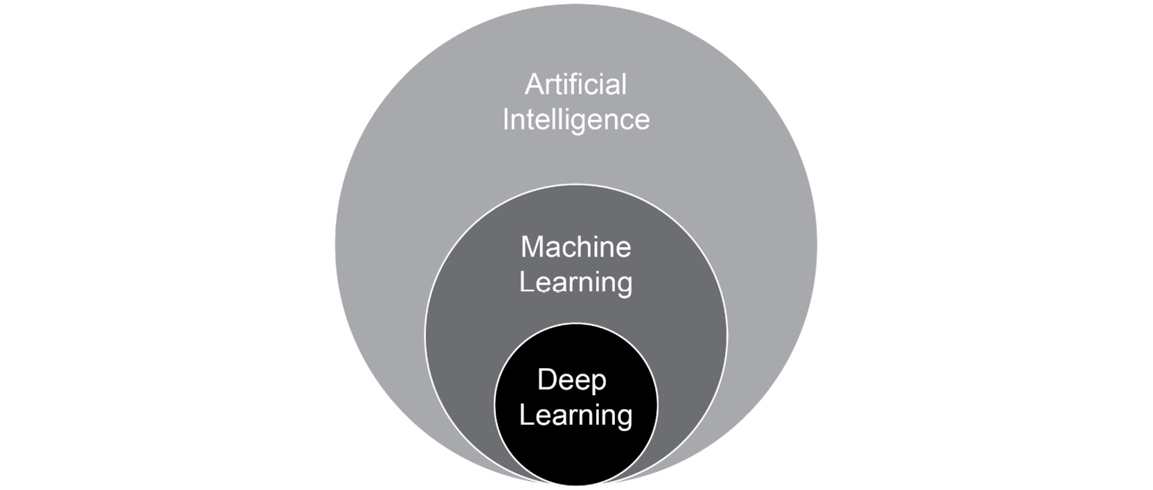
Figure 1.1: Relationship between AI, ML, and DL

Machine Learning

Machine learning is the subset of AI that performs specific tasks by identifying patterns within data and extracting inferences. The inferences that are derived from data are then used to predict outcomes on unseen data. Machine learning differs from traditional computer programming in its approach to solving specific tasks. In traditional computer programming, we write and execute specific business rules and heuristics to get the desired outcomes. However, in machine learning, the rules and heuristics are not explicitly written. These rules and heuristics are learned by providing a dataset. The dataset provided for learning the rules and heuristics is called a training dataset. The whole process of learning and inferring is called training.

Learning rules and heuristics is done using different algorithms that use statistical models for that purpose. These algorithms make use of many representations of data for learning. Each such representation of data is called an example. Each element within an example is called a feature. The following is an example of the famous IRIS dataset (https://archive.ics.uci.edu/ml/datasets/Iris). This dataset is a representation of different species of iris flowers based on different characteristics, such as the length and width of their sepals and petals:

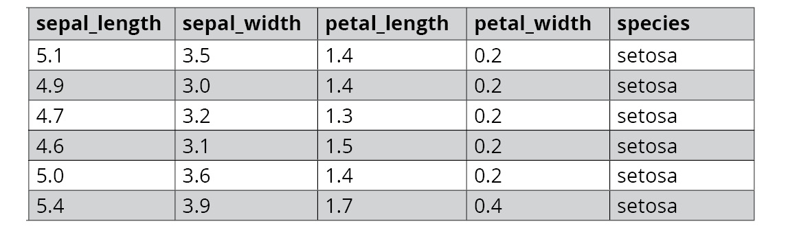
Figure 1.2: Sample data from the IRIS dataset

In the preceding dataset, each row of data represents an example, and each column is a feature. Machine learning algorithms make use of these features to draw inferences from the data. The veracity of the models, and thereby the outcomes that are predicted, depend a lot on the features of the data. If the features provided to the machine learning algorithm are a good representation of the problem statement, the chances of getting a good result are high. Some examples of machine learning algorithms are linear regression, logistic regression, support vector machines, random forest, and XGBoost.

Even though traditional machine learning algorithms are useful for a lot of use cases, they have a lot of dependence on the quality of the features to get superior outcomes. The creation of features is a time-consuming art and requires a lot of domain knowledge. However, even with comprehensive domain knowledge, there are still limitations on transferring that knowledge to derive features, thereby encapsulating the nuances of the data generating processes. Also, with the increasing complexity of the problems that are tackled with machine learning, particularly with the advent of unstructured data (images, voice, text, and so on), it can be almost impossible to create features that represent the complex functions, which, in turn, generate data. As a result, there is often a need to find a different approach to solving complex problems; that is where deep learning comes into play.

Deep Learning

Deep learning is a subset of machine learning and an extension of a certain kind of algorithm called Artificial Neural Networks (ANNs). Neural networks are not a new phenomenon. Neural networks were created in the first half of the 1940s. The development of neural networks was inspired by the knowledge of how the human brain works. Since then, there have been several ups and downs in this field. One defining moment that renewed enthusiasm around neural networks was the introduction of an algorithm called backpropagation by stalwarts in the field such as Geoffrey Hinton. For this reason, Hinton is widely regarded as the 'Godfather of Deep Learning'. We will be discussing neural networks in depth in Chapter 2, Neural Networks.

ANNs with multiple (deep) layers lie at the heart of deep learning. One defining characteristic of deep learning models is their ability to learn features from the input data. Unlike traditional machine learning, where there is the need to create features, deep learning excels in learning different hierarchies of features across multiple layers. Say, for example, we are using a deep learning model to detect faces. The initial layers of the model will learn low-level approximations of a face, such as the edges of the face, as shown in Figure 1.3. Each succeeding layer takes the lower layers' features and puts them together to form more complex features. In the case of face detection, if the initial layer has learned to detect edges, the subsequent layers will put these edges together to form parts of a face such as the nose or eyes. This process continues with each successive layer, with the final layer generating an image of a human face:

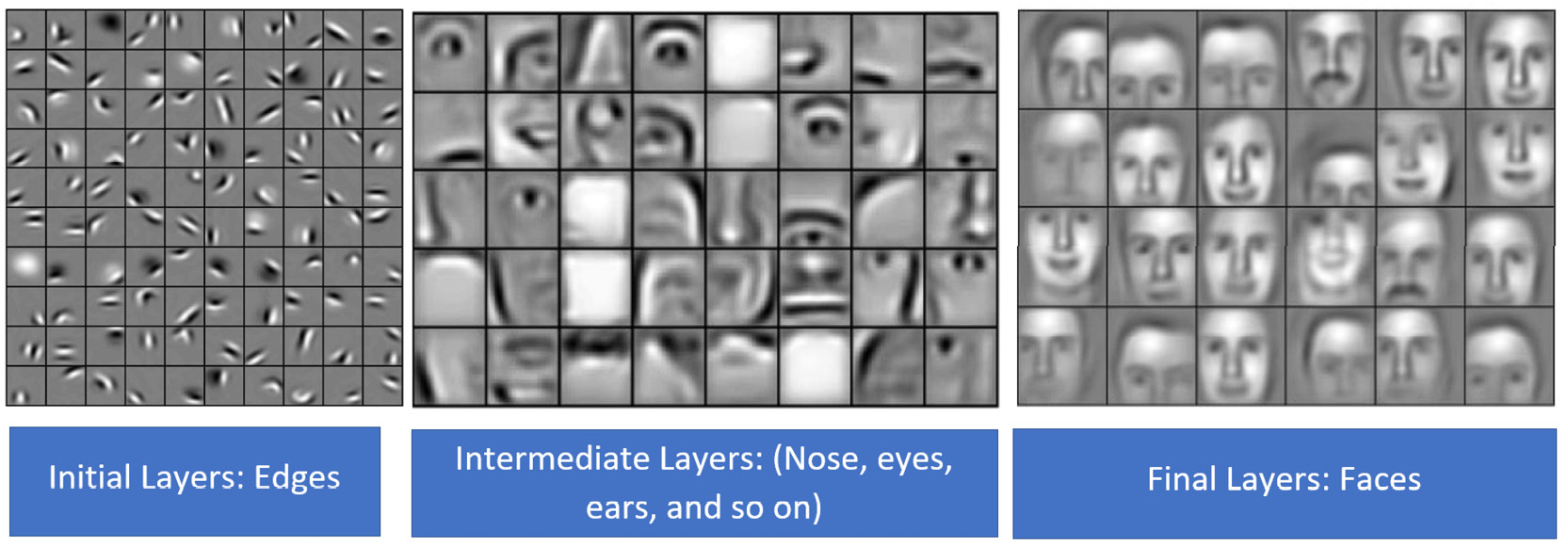
Figure 1.3: Deep learning model for detecting faces

Note

The preceding image is sourced from the popular research paper: Lee, Honglak & Grosse, Roger & Ranganath, Rajesh & Ng, Andrew. (2011). Unsupervised Learning of Hierarchical Representations with Convolutional Deep Belief Networks. Commun. ACM. 54. 95-103. 10.1145/2001269.2001295.

Deep learning techniques have made great strides over the past decade. There are different factors that have led to the exponential rise of deep learning techniques. At the top of the list is the availability of large quantities of data. The digital age, with its increasing web of connected devices, has generated lots of data, especially unstructured data. This, in turn, has fueled the large-scale adoption of deep learning techniques as they are well-suited to handle large unstructured data.

Another major factor that has led to the rise in deep learning is the strides that have been made in computing infrastructure. Deep learning models that have large numbers of layers and millions of parameters necessitate great computing power. The advances in computing layers such as Graphical Processing Units (GPUs) and Tensor Processing Units (TPUs) at an affordable cost has led to the large-scale adoption of deep learning.

The pervasiveness of deep learning was also accelerated by open sourcing different frameworks in order to build and implement deep learning models. In 2015, the Google Brain team open sourced the TensorFlow framework and since then TensorFlow has grown to be one of the most popular frameworks for deep learning. The other major frameworks available are PyTorch, MXNet, and Caffe. We will be using the TensorFlow framework in this book.

Before we dive deep into the building blocks of deep learning, let's get our hands dirty with a quick demo that illustrates the power of deep learning models. You don't need to know any of the code that is presented in this demo. Simply follow the instructions and you'll be able to get a quick glimpse of the basic capabilities of deep learning.

Using Deep Learning to Classify an Image

In the exercise that follows, we will classify an image of a pizza and convert the resulting class text into speech. To classify the image, we will be using a pre-trained model. The conversion of text into speech will be done using a freely available API called Google Text-to-Speech (gTTS). Before we get into it, let's understand some of the key building blocks of this demo.

Pre-Trained Models

Training a deep learning model requires a lot of computing infrastructure and time, with big datasets. However, to aid with research and learning, the deep learning community has also made models that have been trained on large datasets available. These pre-trained models can be downloaded and used for predictions or can be used for further training. In this demo, we will be using a pre-trained model called ResNet50. This model is available along with the Keras package. This pre-trained model can predict 1,000 different classes of objects that we encounter in our daily lives, such as birds, animals, automobiles, and more.

The Google Text-to-Speech API

Google has made its Text-to-Speech algorithm available for limited use. We will be using this algorithm to convert the predicted text into speech.

Prerequisite Packages for the Demo

For this demo to work, you will need the following packages installed on your machine:

• TensorFlow 2.0
• Keras
• gTTS

Please refer to the Preface to understand the process of installing the first two packages. Installing gTTS will be shown in the exercise. Let's dig into the demo.

Exercise 1.01: Image and Speech Recognition Demo

In this exercise, we will demonstrate image recognition and speech-to-text conversion using deep learning models. At this point, you will not be able to understand each and every line of the code. This will be explained later. For now, just execute the code and find out how easy it is to build deep learning and AI applications with TensorFlow. Follow these steps to complete this exercise:

1. Open a Jupyter Notebook and name it Exercise 1.01. For details on how to start a Jupyter Notebook, please refer to the preface.
2. Import all the required libraries:

   from tensorflow.keras.preprocessing.image import load_img
   from tensorflow.keras.preprocessing.image import img_to_array
   from tensorflow.keras.applications.resnet50 import ResNet50
   from tensorflow.keras.preprocessing import image
   from tensorflow.keras.applications.resnet50 \
   import preprocess_input
   from tensorflow.keras.applications.resnet50 \
   import decode_predictions

   Note

   The code snippet shown here uses a backslash ( \ ) to split the logic across multiple lines. When the code is executed, Python will ignore the backslash, and treat the code on the next line as a direct continuation of the current line.

   Here is a brief description of the packages we'll be importing:

   load_img: Loads the image into the Jupyter Notebook

   img_to_array: Converts the image into a NumPy array, which is the desired format for Keras

   preprocess_input: Converts the input into a format that's acceptable for the model

   decode_predictions: Converts the numeric output of the model prediction into text labels

   Resnet50: This is the pre-trained image classification model

3. Create an instance of the pre-trained Resnet model:

   mymodel = ResNet50()

   You should get a message similar to the following as it downloads:

   Figure 1.4: Loading Resnet50

   Resnet50 is a pre-trained image classification model. For first-time users, it will take some time to download the model into your environment.

4. Download an image of a pizza from the internet and store it in the same folder that you are running the Jupyter Notebook in. Name the image im1.jpg.

   Note

   You can also use the image we are using by downloading it from this link: https://packt.live/2AHTAC9

5. Load the image to be classified using the following command:

   myimage = load_img('im1.jpg', target_size=(224, 224))

   If you are storing the image in another folder, the complete path of the location where the image is located has to be given in place of the im1.jpg command. For example, if the image is stored in D:/projects/demo, the code should be as follows:

   myimage = load_img('D:/projects/demo/im1.jpg', \
                      target_size=(224, 224))

6. Let's display the image using the following command:

   myimage

   The output of the preceding command will be as follows:

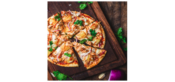
   Figure 1.5: Output displayed after loading the image

7. Convert the image into a numpy array as the model expects it in this format:

   myimage = img_to_array(myimage)

8. Reshape the image into a four-dimensional format since that's what is expected by the model:

   myimage = myimage.reshape((1, 224, 224, 3))

9. Prepare the image for submission by running the preprocess_input() function:

   myimage = preprocess_input(myimage)

10. Run the prediction:

    myresult = mymodel.predict(myimage)

11. The prediction results in a number that needs to be converted into the corresponding label in text format:

    mylabel = decode_predictions(myresult)

12. Next, type in the following code to display the label:

    mylabel = mylabel[0][0]

13. Print the label using the following code:

    print("This is a : " + mylabel[1])

    If you have followed the steps correctly so far, the output will be as follows:

    This is a : pizza

    The model has successfully identified our image. Interesting, isn't it? In the next few steps, we'll take this a step further and convert this result into speech.

    Tip

    While we have used an image of a pizza here, you can use just about any image with this model. We urge you to try out this exercise multiple times with different images.

14. Prepare the text to be converted into speech:

    sayit="This is a "+mylabel[1]

15. Install the gtts package, which is required for converting text into speech. This can be implemented in the Jupyter Notebook, as follows:

    !pip install gtts

16. Import the required libraries:

    from gtts import gTTS
    import os

    The preceding code will import two libraries. One is gTTS, that is, Google Text-to-Speech, which is a cloud-based open source API for converting text into speech. Another is the os library that is used to play the resulting audio file.

17. Call the gTTS API and pass the text as a parameter:

    myobj = gTTS(text=sayit)

    Note

    You need to be online while running the preceding step.

18. Save the resulting audio file. This file will be saved in the home directory where the Jupyter Notebook is being run.

    myobj.save("prediction.mp3")

    Note

    You can also specify the path where you want it to be saved by including the absolute path in front of the name; for example, (myobj.save('D:/projects/prediction.mp3').

19. Play the audio file:

    os.system("prediction.mp3")

    If you have correctly followed the preceding steps, you will hear the words This is a pizza being spoken.

    Note

    To access the source code for this specific section, please refer to https://packt.live/2ZPZx8B.

    You can also run this example online at https://packt.live/326cRIu. You must execute the entire Notebook in order to get the desired result.

In this exercise, we learned how to build a deep learning model by making use of publicly available models using a few lines of code in TensorFlow. Now that you have got a taste of deep learning, let's move forward and learn about the different building blocks of deep learning.

Deep Learning Models

At the heart of most of the popular deep learning models are ANNs, which are inspired by our knowledge of how the brain works. Even though no single model can be called perfect, different models perform better in different scenarios. In the sections that follow, we will learn about some of the most prominent models.

The Multi-Layer Perceptron

The multi-layer perceptron (MLP) is a basic type of neural network. An MLP is also known as a feed-forward network. A representation of an MLP can be seen in the following figure:

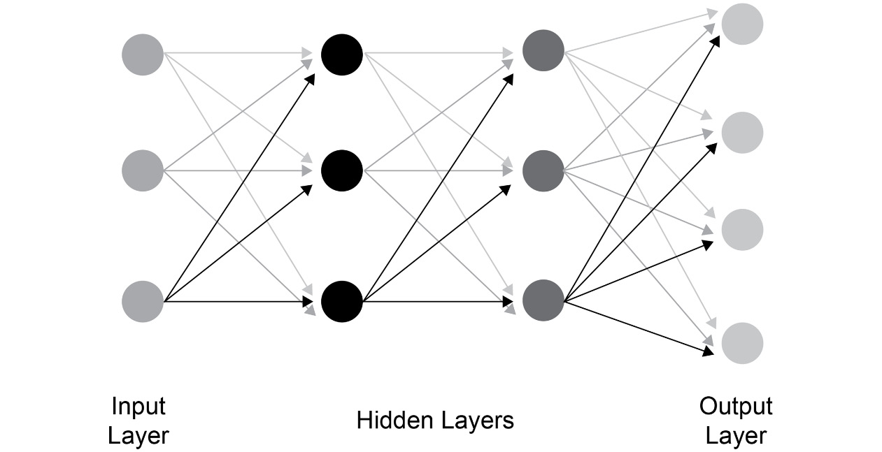
Figure 1.6: MLP representation

One of the basic building blocks of an MLP (or any neural network) is a neuron. A network consists of multiple neurons connected to successive layers. At a very basic level, an MLP will consist of an input layer, a hidden layer, and an output layer. The input layer will have neurons equal to the input data. Each input neuron will have a connection to all the neurons of the hidden layer. The final hidden layer will be connected to the output layer. The MLP is a very useful model and can be tried out on various classification and regression problems. The concept of an MLP will be covered in detail in Chapter 2, Neural Networks.

Convolutional Neural Networks

A convolutional neural network (CNN) is a class of deep learning model that is predominantly used for image recognition. When we discussed the MLP, we saw that each neuron in a layer is connected to every other neuron in the subsequent layer. However, CNNs adopt a different approach and do not resort to such a fully connected architecture. Instead, CNNs extract local features from images, which are then fed to the subsequent layers.

CNNs rose to prominence in 2012 when an architecture called AlexNet won a premier competition called the ImageNet Large-Scale Visual Recognition Challenge (ILSVRC). ILSVRC is a large-scale computer vision competition where teams from around the globe compete for the prize of the best computer vision model. Through the 2012 research paper titled ImageNet Classification with Deep Convolutional Neural Networks (https://papers.nips.cc/paper/4824-imagenet-classification-with-deep-convolutional-neural-networks), Alex Krizhevsky, et al. (University of Toronto) showcased the true power of CNN architectures, which eventually won them the 2012 ILSVRC challenge. The following figure depicts the structure of the AlexNet model, a CNN model whose high performance catapulted CNNs to prominence in the deep learning domain. While the structure of this model may look complicated to you, in Chapter 3, Image Classification with Convolutional Neural Networks, the working of such CNN networks will be explained to you in detail:

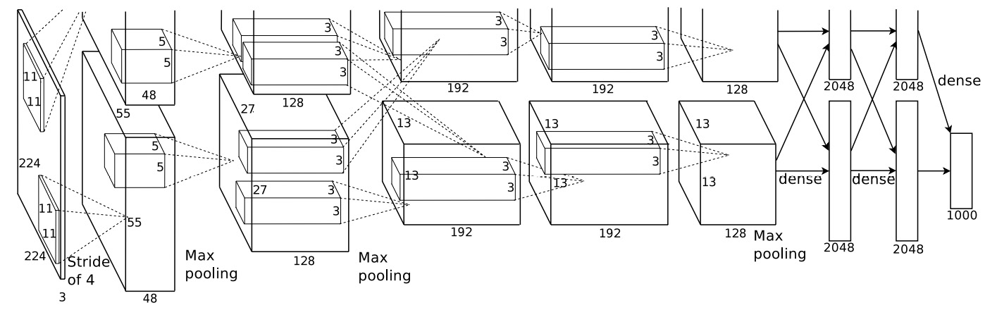
Figure 1.7: CNN architecture of the AlexNet model

Note

The aforementioned diagram is sourced from the popular research paper: Krizhevsky, Alex & Sutskever, Ilya & Hinton, Geoffrey. (2012). ImageNet Classification with Deep Convolutional Neural Networks. Neural Information Processing Systems. 25. 10.1145/3065386.

Since 2012, there have been many breakthrough CNN architectures expanding the possibilities for computer vision. Some of the prominent architectures are ZFNet, Inception (GoogLeNet), VGG, and ResNet.

Some of the most prominent use cases where CNNs are put to use are as follows:

• Image recognition and optical character recognition (OCR)
• Face recognition on social media
• Text classification
• Object detection for self-driving cars
• Image analysis for health care

Another great benefit of working with deep learning is that you needn't always build your models from scratch – you could use models built by others and use them for your own applications. This is known as "transfer learning", and it allows you to benefit from the active deep learning community.

We will apply transfer learning to image processing and learn about CNNs and their dynamics in detail in Chapter 3, Image Classification with Convolutional Neural Networks.

Recurrent Neural Networks

In traditional neural networks, the inputs are independent of the outputs. However, in cases such as language translation, where there is dependence on the words preceding and succeeding a word, there is a need to understand the dynamics of the sequences in which words appear. This problem was solved by a class of networks called recurrent neural networks (RNNs). RNNs are a class of deep learning networks where the output from the previous step is sent as input to the current step. A distinct characteristic of an RNN is a hidden layer, which remembers the information of other inputs in a sequence. A high-level representation of an RNN can be seen in the following figure. You'll learn more about the inner workings of these networks in Chapter 5, Deep Learning for Sequences:

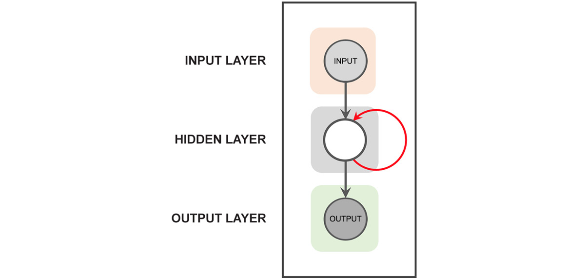
Figure 1.8: Structure of RNNs

There are different types of RNN architecture. Some of the most prominent ones are long short-term memory (LSTM) and gated recurrent units (GRU).

Some of the important use cases for RNNs are as follows:

• Language modeling and text generation
• Machine translation
• Speech recognition
• Generating image descriptions

RNNs will be covered in detail in Chapter 5, Deep Learning for Sequences, and Chapter 6, LSTMs, GRUs, and Advanced RNNs.

Generative Adversarial Networks

Generative adversarial networks (GANs) are networks that are capable of generating data distributions similar to any real data distributions. One of the pioneers of deep learning, Yann LeCun, described GANs as one of the most promising ideas in deep learning in the last decade.

To give you an example, suppose we want to generate images of dogs from random noise data. For this, we train a GAN network with real images of dogs and the noise data until we generate data that looks like the real images of dogs. The following diagram explains the concept behind GANs. At this stage, you might not fully understand this concept. It will be explained in detail in Chapter 7, Generative Adversarial Networks.

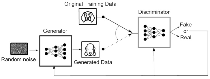
Figure 1.9: Structure of GANs

Note

The aforementioned diagram is sourced from the popular research paper: Barrios, Buldain, Comech, Gilbert & Orue (2019). Partial Discharge Classification Using Deep Learning Methods—Survey of Recent Progress (https://doi.org/10.3390/en12132485).

GANs are a big area of research, and there are many use cases for them. Some of the useful applications of GANs are as follows:

• Image translation
• Text to image synthesis
• Generating videos
• The restoration of art

GANs will be covered in detail in Chapter 7, Generative Adversarial Networks.

The possibilities and promises of deep learning are huge. Deep learning applications have become ubiquitous in our daily lives. Some notable examples are as follows:

• Chatbots
• Robots
• Smart speakers (such as Alexa)
• Virtual assistants
• Recommendation engines
• Drones
• Self-driving cars or autonomous vehicles

This ever-expanding canvas of possibilities makes it a great toolset in the arsenal of a data scientist. This book will progressively introduce you to the amazing world of deep learning and make you adept at applying it to real-world scenarios.

TensorFlow is a deep learning library developed by Google. At the time of writing this book, TensorFlow is by far the most popular deep learning library. It was originally developed by a team within Google called the Google Brain team for their internal use and was subsequently open sourced in 2015. The Google Brain team has developed popular applications such as Google Photos and Google Cloud Speech-to-Text, which are deep learning applications based on TensorFlow. TensorFlow 1.0 was released in 2017, and within a short period of time, it became the most popular deep learning library ahead of other existing libraries, such as Caffe, Theano, and PyTorch. It is considered the industry standard, and almost every organization that is doing something in the deep learning space has adopted it. Some of the key features of TensorFlow are as follows:

• It can be used with all common programming languages, such as Python, Java, and R
• It can be deployed on multiple platforms, including Android and Raspberry Pi
• It can run in a highly distributed mode and hence is highly scalable

After being in Alpha/Beta release for a long time, the final version of TensorFlow 2.0 was released on September 30, 2019. The focus of TF2.0 was to make the development of deep learning applications easier. Let's go ahead and understand the basics of the TensorFlow 2.0 framework.

Tensors

Inside the TensorFlow program, every data element is called a tensor. A tensor is a representation of vectors and matrices in higher dimensions. The rank of a tensor denotes its dimensions. Some of the common data forms represented as tensors are as follows.

Scalar

A scalar is a tensor of rank 0, which only has magnitude.

For example, [ 12 ] is a scalar of magnitude 12.

Vector

A vector is a tensor of rank 1.

For example, [ 10 , 11, 12, 13].

Matrix

A matrix is a tensor of rank 2.

For example, [ [10,11] , [12,13] ]. This tensor has two rows and two columns.

Tensor of rank 3

This is a tensor in three dimensions. For example, image data is predominantly a three-dimensional tensor with width, height, and the number of channels as its three dimensions. The following is an example of a tensor with three dimensions, that is, it has two rows, three columns, and three channels:

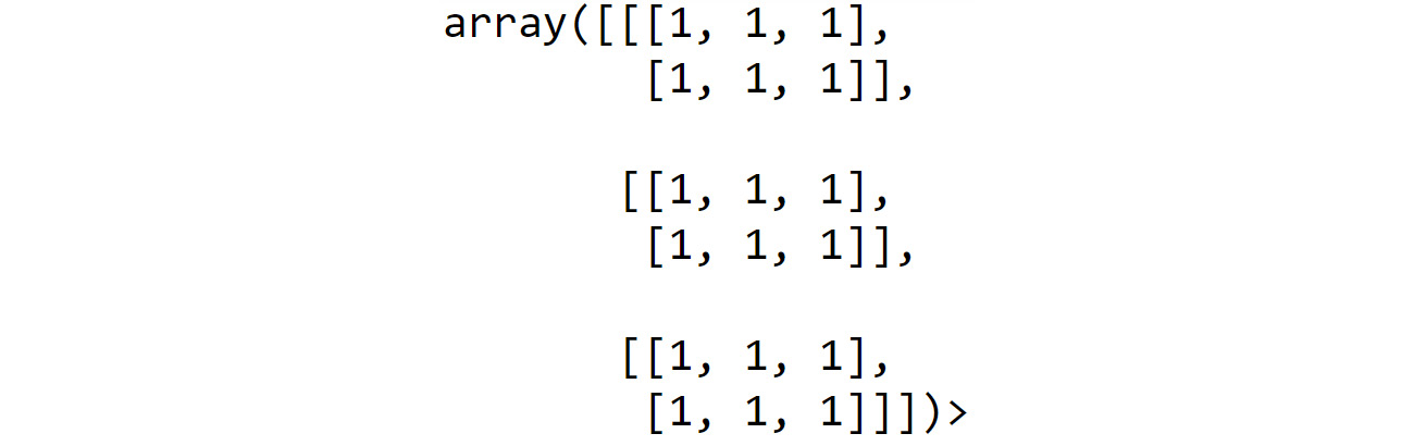
Figure 1.10: Tensor with three dimensions

The shape of a tensor is represented by an array and indicates the number of elements in each dimension. For example, if the shape of a tensor is [2,3,5], it means the tensor has three dimensions. If this were to be image data, this shape would mean that this tensor has two rows, three columns, and five channels. We can also get the rank from the shape. In this example, the rank of the tensor is three, since there are three dimensions. This is further illustrated in the following diagram:

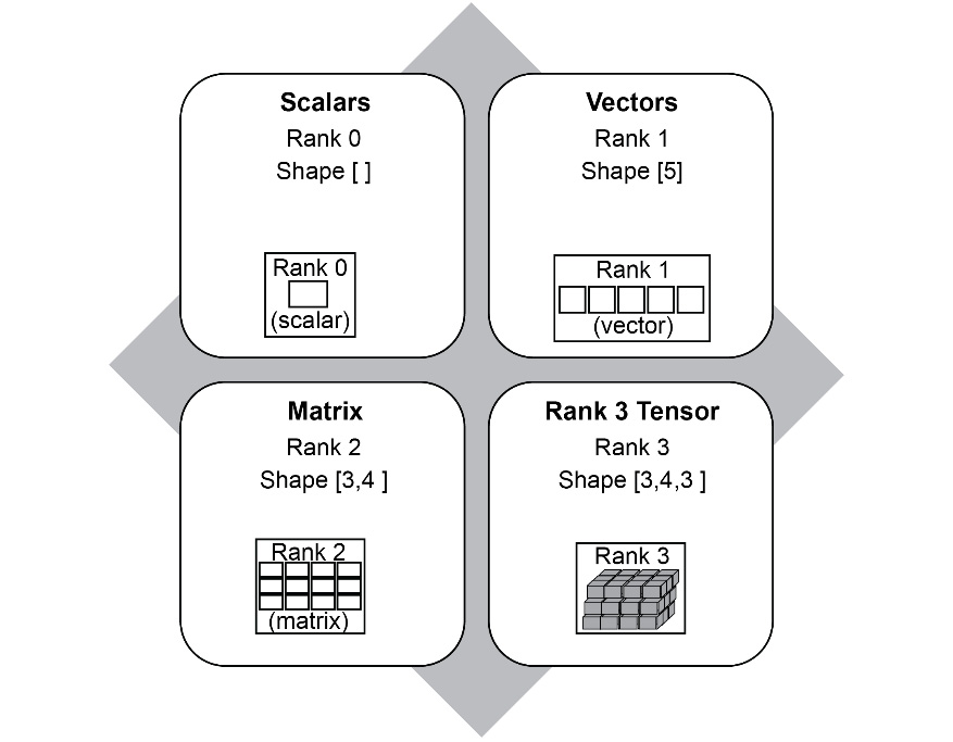
Figure 1.11: Examples of Tensor rank and shape

Constants

Constants are used to store values that are not changed or modified during the course of the program. There are multiple ways in which a constant can be created, but the simplest way is as follows:

a = tf.constant (10)

This creates a tensor initialized to 10. Keep in mind that a constant's value cannot be updated or modified by reassigning a new value to it. Another example is as follows:

s = tf.constant("Hello")

In this line, we are instantiating a string as a constant.

Variables

A variable is used to store data that can be updated and modified during the course of the program. We will look at this in more detail in Chapter 2, Neural Networks. There are multiple ways of creating a variable, but the simplest way is as follows:

b=tf.Variable(20)

In the preceding code, the variable b is initialized to 20. Note that in TensorFlow, unlike constants, the term Variable is written with an uppercase V.

A variable can be reassigned a different value during the course of the program. Variables can be used to assign any type of object, including scalars, vectors, and multi-dimensional arrays. The following is an example of how an array whose dimensions are 3 x 3 can be created in TensorFlow:

C = tf.Variable([[1,2,3],[4,5,6],[7,8,9]])

This variable can be initialized to a 3 x 3 matrix, as follows:

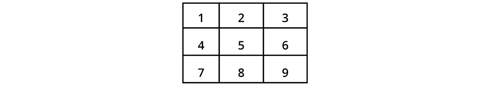
Figure 1.12: 3 x 3 matrix

Now that we know some of the basic concepts of TensorFlow, let's learn how to put them into practice.

Defining Functions in TensorFlow

A function can be created in Python using the following syntax:

def myfunc(x,y,c):
    Z=x*x*y+y+c
    return Z

A function is initiated using the special operator def, followed by the name of the function, myfunc, and the arguments for the function. In the preceding example, the body of the function is in the second line, and the last line returns the output.

In the following exercise, we will learn how to implement a small function using the variables and constants we defined earlier.

Exercise 1.02: Implementing a Mathematical Equation

In this exercise, we will solve the following mathematical equation using TensorFlow:

Figure 1.13: Mathematical equation to be solved using TensorFlow

We will use TensorFlow to solve it, as follows:

X=3
Y=4

While there are multiple ways of doing this, we will only explore one of the ways in this exercise. Follow these steps to complete this exercise:

1. Open a new Jupyter Notebook and rename it Exercise 1.02.
2. Import the TensorFlow library using the following command:

   import tensorflow as tf

3. Now, let's solve the equation. For that, you will need to create two variables, X and Y, and initialize them to the given values of 3 and 4, respectively:

   X=tf.Variable(3)
   Y=tf.Variable(4)

4. In our equation, the value of 2 isn't changing, so we'll store it as a constant by typing the following code:

   C=tf.constant(2)

5. Define the function that will solve our equation:

   def myfunc(x,y,c):
       Z=x*x*y+y+c
       return Z

6. Call the function by passing X, Y, and C as parameters. We'll be storing the output of this function in a variable called result:

   result=myfunc(X,Y,C)

7. Print the result using the tf.print() function:

   tf.print(result)

   The output will be as follows:

   42

   Note

   To access the source code for this specific section, please refer to https://packt.live/2ClXKjj.

   You can also run this example online at https://packt.live/2ZOIN1C. You must execute the entire Notebook in order to get the desired result.

In this exercise, we learned how to define and use a function. Those familiar with Python programming will notice that it is not a lot different from normal Python code.

In the rest of this chapter, we will prepare ourselves by looking at some basic linear algebra and familiarize ourselves with some of the common vector operations, so that understanding neural networks in the next chapter will be much easier.

Linear Algebra with TensorFlow

The most important linear algebra topic that will be used in neural networks is matrix multiplication. In this section, we will explain how matrix multiplication works and then use TensorFlow's built-in functions to solve some matrix multiplication examples. This is essential in preparation for neural networks in the next chapter.

How does matrix multiplication work? You might have studied this as part of high school, but let's do a quick recap.

Let's say we have to perform a matrix multiplication between two matrices, A and B, where we have the following:

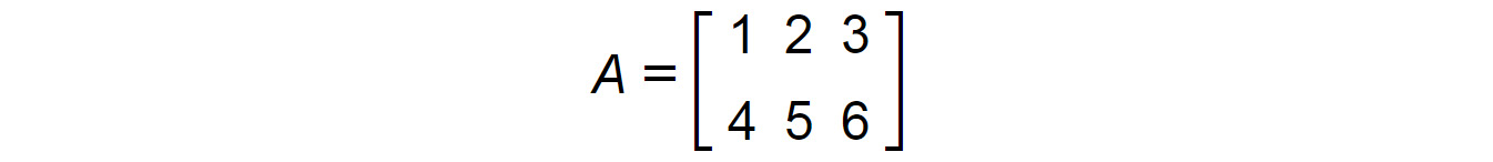
Figure 1.14: Matrix A

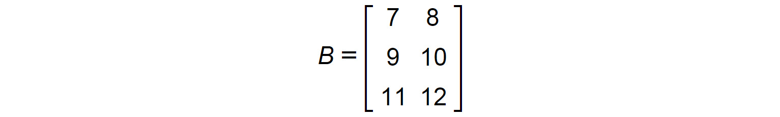
Figure 1.15: Matrix B

The first step would be to check whether multiplying a 2 x 3 matrix by a 3 x 2 matrix is possible. There is a prerequisite for matrix multiplication. Remember that C=R, that is, the number of columns (C) in the first matrix should be equal to the number of rows (R) in the second matrix. And remember the sequence matters here, and that's why, A x B is not equal to B x A. In this example, C=3 and R=3. So, multiplication is possible.

The resultant matrix would have the number of rows equal to that in A and the number of columns equal to that in B. So, in this case, the result would be a 2 x 2 matrix.

To begin multiplying the two matrices, take the elements of the first row of A (R1) and the elements of the first column of B (C1):

Figure 1.16: Matrix A(R1)

Figure 1.17: Matrix B(C1)

Get the sum of the element-wise products, that is, (1 x 7) + (2 x 9) + (3 x 11) = 58. This will be the first element in the resultant 2 x 2 matrix. We'll call this incomplete matrix D(i) for now:

Figure 1.18: Incomplete matrix D(i)

Repeat this with the first row of A(R1) and the second column of B (C2):

Figure 1.19: First row of matrix A

Figure 1.20: Second column of matrix B

Get the sum of the products of the corresponding elements, that is, (1 x 8) + (2 x 10) + (3 x 12) = 64. This will be the second element in the resultant matrix:

Figure 1.21: Second element of matrix D(i)

Repeat the same with the second row to get the final result:

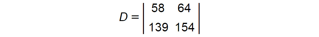
Figure 1.22: Matrix D

The same matrix multiplication can be performed in TensorFlow using a built-in method called tf.matmul(). The matrices that need to be multiplied must be supplied to the model as variables, as shown in the following example:

C = tf.matmul(A,B)

In the preceding case, A and B are the matrices that we want to multiply. Let's practice this method by using TensorFlow to multiply the two matrices we multiplied manually.

Exercise 1.03: Matrix Multiplication Using TensorFlow

In this exercise, we will use the tf.matmul() method to multiply two matrices using tensorflow. Follow these steps to complete this exercise:

1. Open a new Jupyter Notebook and rename it Exercise 1.03.
2. Import the tensorflow library and create two variables, X and Y, as matrices. X is a 2 x 3 matrix and Y is a 3 x 2 matrix:

   import tensorflow as tf
   X=tf.Variable([[1,2,3],[4,5,6]])
   Y=tf.Variable([[7,8],[9,10],[11,12]])

3. Print and display the values of X and Y to make sure the matrices are created correctly. We'll start by printing the value of X:

   tf.print(X)

   The output will be as follows:

   [[1 2 3]
    [4 5 6]]

   Now, let's print the value of Y:

   tf.print(Y)

   The output will be as follows:

   [[7 8]
    [9 10]
    [11 12]]

4. Perform matrix multiplication by calling the TensorFlow tf.matmul() function:

   c1=tf.matmul(X,Y)

   To display the result, print the value of c1:

   tf.print(c1)

   The output will be as follows:

   [[58 64]
    [139 154]]

5. Let's perform matrix multiplication by changing the order of the matrices:

   c2=tf.matmul(Y,X)

   To display the result, let's print the value of c2:

   tf.print(c2)

   The resulting output will be as follows.

   [[39 54 69]
    [49 68 87]
    [59 82 105]]

   Note that the results are different since we changed the order.

   Note

   To access the source code for this specific section, please refer to https://packt.live/3eevyw4.

   You can also run this example online at https://packt.live/2CfGGvE. You must execute the entire Notebook in order to get the desired result.

In this exercise, we learned how to create matrices in TensorFlow and how to perform matrix multiplication. This will come in handy when we create our own neural networks.

The reshape Function

Reshape, as the name suggests, changes the shape of a tensor from its current shape to a new shape. For example, you can reshape a 2 × 3 matrix to a 3 × 2 matrix, as shown here:

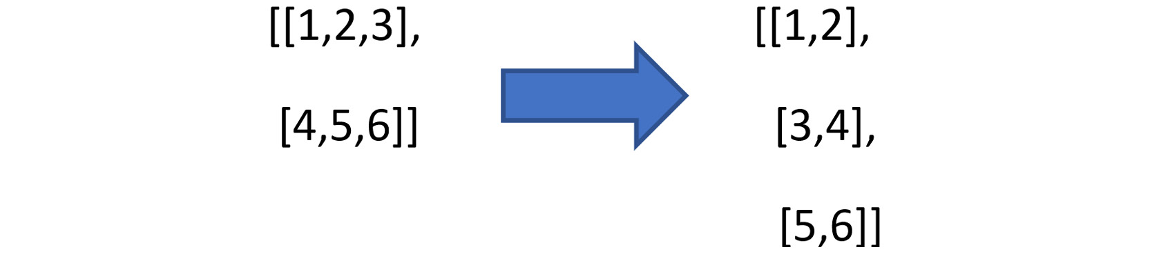
Figure 1.23: Reshaped matrix

Let's consider the following 2 × 3 matrix, which we defined as follows in the previous exercise:

X=tf.Variable([[1,2,3],[4,5,6]])

We can print the shape of the matrix using the following code:

X.shape

From the following output, we can see the shape, which we already know:

TensorShape([2, 3])

Now, to reshape X into a 3 × 2 matrix, TensorFlow provides a handy function called tf.reshape(). The function is implemented with the following arguments:

tf.reshape(X,[3,2])

In the preceding code, X is the matrix that needs to be reshaped, and [3,2] is the new shape that the X matrix has to be reshaped to.

Reshaping matrices is a handy operation when implementing neural networks. For example, a prerequisite when working with images using CNNs is that the image has to be of rank 3, that is, it has to have three dimensions: width, height, and depth. If our image is a grayscale image that has only two dimensions, the reshape operation will come in handy to add a third dimension. In this case, the third dimension will be 1:

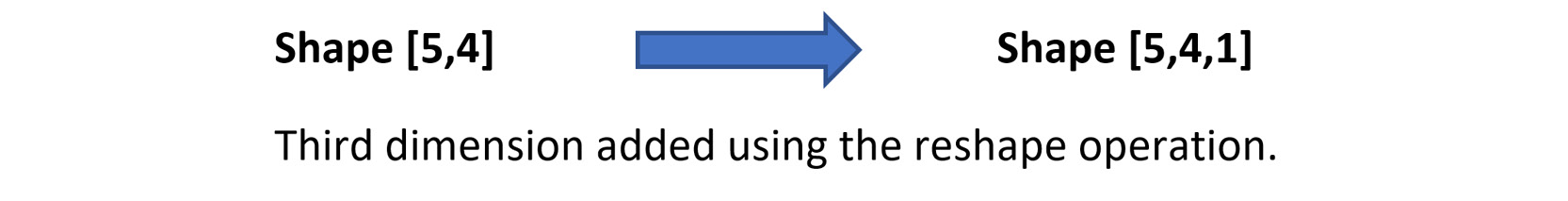
Figure 1.24: Changing the dimension using reshape()

In the preceding figure, we are reshaping a matrix of shape [5,4] to a matrix of shape [5,4,1]. In the exercise that follows, we will be using the reshape() function to reshape a [5,4] matrix.

There are some important considerations when implementing the reshape() function:

• The total number of elements in the new shape should be equal to the total number of elements in the original shape. For example, you can reshape a 2 × 3 matrix (a total of 6 elements) to a 3 × 2 matrix since the new shape also has 6 elements. However, you cannot reshape it to 3 × 3 or 3 × 4.
• The reshape() function should not be confused with transpose(). In reshape(), the sequence of the elements of the matrix is retained and the elements are rearranged in the new shape in the same sequence. However, in the case of transpose(), the rows become columns and the columns become rows. Hence the sequence of the elements will change.
• The reshape() function will not change the original matrix unless you assign the new shape to it. Otherwise, it simply displays the new shape without actually changing the original variable. For example, let's say x has shape [2,3] and you simply run tf.reshape(x,[3,2]). When you check the shape of x again, it will remain as [2,3]. In order to actually change the shape, you need to assign the new shape to it, like this:

  x=tf.reshape(x,[3,2])

Let's try implementing reshape() in TensorFlow in the exercise that follows.

Exercise 1.04: Reshaping Matrices Using the reshape() Function in TensorFlow

In this exercise, we will reshape a [5,4] matrix into the shape of [5,4,1] using the reshape() function. This exercise will help us understand how reshape() can be used to change the rank of a tensor. Follow these steps to complete this exercise:

1. Open a Jupyter Notebook and rename it Exercise 1.04. Then, import tensorflow and create the matrix we want to reshape:

   import tensorflow as tf
   A=tf.Variable([[1,2,3,4], \
                  [5,6,7,8], \
                  [9,10,11,12], \
                  [13,14,15,16], \
                  [17,18,19,20]])

2. First, we'll print the variable A to check whether it is created correctly, using the following command:

   tf.print(A)

   The output will be as follows:

   [[1 2 3 4]
    [5 6 7 8]
    [9 10 11 12]
    [13 14 15 16]
    [17 18 19 20]]

3. Let's print the shape of A, just to be sure:

   A.shape

   The output will be as follows:

   TensorShape([5, 4])

   Currently, it has a rank of 2. We'll be using the reshape() function to change its rank to 3.

4. Now, we will reshape A to the shape [5,4,1] using the following command. We've thrown in the print command just to see what the output looks like:

   tf.print(tf.reshape(A,[5,4,1]))

   We'll get the following output:

   [[[1]
     [2]
     [3]
     [4]]
    [[5]
     [6]
     [7]
     [8]]
    [[9]
     [10]
     [11]
     [12]]
    [[13]
     [14]
     [15]
     [16]]
    [[17]
     [18]
     [19]
     [20]]]

   That worked as expected.

5. Let's see the new shape of A:

   A.shape

   The output will be as follows:

   TensorShape([5, 4])

   We can see that A still has the same shape. Remember that we discussed that in order to save the new shape, we need to assign it to itself. Let's do that in the next step.

6. Here, we'll assign the new shape to A:

   A = tf.reshape(A,[5,4,1])

7. Let's check the new shape of A once again:

   A.shape

   We will see the following output:

   TensorShape([5, 4, 1])

   With that, we have not just reshaped the matrix but also changed its rank from 2 to 3. In the next step, let's print out the contents of A just to be sure.

8. Let's see what A contains now:

   tf.print(A)

   The output, as expected, will be as follows:

   [[[1]
     [2]
     [3]
     [4]]
    [[5]
     [6]
     [7]
     [8]]
    [[9]
     [10]
     [11]
     [12]]
    [[13]
     [14]
     [15]
     [16]]
    [[17]
     [18]
     [19]
     [20]]]

   Note

   To access the source code for this specific section, please refer to https://packt.live/3gHvyGQ.

   You can also run this example online at https://packt.live/2ZdjdUY. You must execute the entire Notebook in order to get the desired result.

In this exercise, we saw how to use the reshape() function. Using reshape(), we can change the rank and shape of tensors. We also learned that reshaping a matrix changes the shape of the matrix without changing the order of the elements within the matrix. Another important thing that we learned was that the reshape dimension has to align with the number of elements in the matrix. Having learned about the reshape function, we will go ahead and learn about the next function, which is Argmax.

The argmax Function

Now, let's understand the argmax function, which is frequently used in neural networks. Argmax returns the position of the maximum value along a particular axis in a matrix or tensor. It must be noted that it does not return the maximum value, but rather the index position of the maximum value.

For example, if x = [1,10,3,5], then tf.argmax(x) will return 1 since the maximum value (which in this case is 10) is in the index position 1.

Note

In Python, the index starts with 0. So, considering the preceding example of x, the element 1 will have an index of 0, 10 will have an index of 1, and so on.

Now, let's say we have the following:

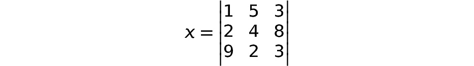
Figure 1.25: An example matrix

In this case, argmax has to be used with the axis parameter. When axis equals 0, it returns the position of the maximum value in each column, as shown in the following figure:

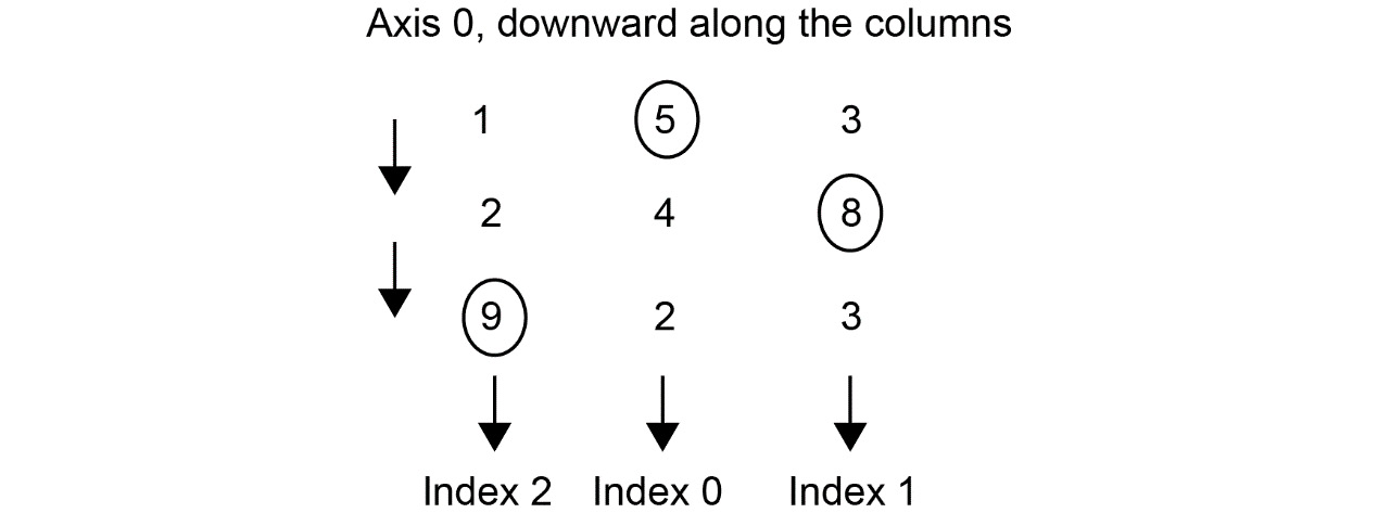
Figure 1.26: The argmax operation along axis 0

As you can see, the maximum value in the first column is 9, so the index, in this case, will be 2. Similarly, if we move along to the second column, the maximum value is 5, which has an index of 0. In the third column, the maximum value is 8, and hence the index is 1. If we were to run the argmax function on the preceding matrix with the axis as 0, we would get the following output:

[2,0,1]

When axis = 1, argmax returns the position of the maximum value across each row, like this:

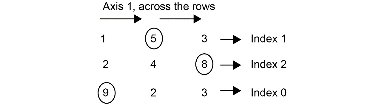
Figure 1.27: The argmax operation along axis 1

Moving along the rows, we have 5 at index 1, 8 at index 2, and 9 at index 0. If we were to run the argmax function on the preceding matrix with the axis as 1, we would get the following output:

[1,2,0]

With that, let's try and implement argmax on a matrix.

Exercise 1.05: Implementing the argmax() Function

In this exercise, we are going to use the argmax function to find the position of the maximum value in a given matrix along axes 0 and 1. Follow these steps to complete this exercise:

1. Import tensorflow and create the following matrix:

   import tensorflow as tf
   X=tf.Variable([[91,12,15], [11,88,21],[90, 87,75]])

2. Let's print X and see what the matrix looks like:

   tf.print(X)

   The output will be as follows:

   [[91 12 15]
    [11 88 21]
    [90 87 75]]

3. Print the shape of X:

   X.shape

   The output will be as follows:

   TensorShape([3, 3])

4. Now, let's use argmax to find the positions of the maximum values while keeping axis as 0:

   tf.print(tf.argmax(X,axis=0))

   The output will be as follows:

   [0 1 2]

   Referring to the matrix in Step 2, we can see that, moving across the columns, the index of the maximum value (91) in the first column is 0. Similarly, the index of the maximum value along the second column (88) is 1. And finally, the maximum value across the third column (75) has index 2. Hence, we have the aforementioned output.

5. Now, let's change the axis to 1:

   tf.print(tf.argmax(X,axis=1))

   The output will be as follows:

   [0 1 0]

Again, referring to the matrix in Step 2, if we move along the rows, the maximum value along the first row is 91, which is at index 0. Similarly, the maximum value along the second row is 88, which is at index 1. Finally, the third row is at index 0 again, with a maximum value of 75.

Note

To access the source code for this specific section, please refer to https://packt.live/2ZR5q5p.

You can also run this example online at https://packt.live/3eewhNO. You must execute the entire Notebook in order to get the desired result.

In this exercise, we learned how to use the argmax function to find the position of the maximum value along a given axis of a tensor. This will be used in the subsequent chapters when we perform classification using neural networks.

Optimizers

Before we look at neural networks, let's learn about one more important concept, and that is optimizers. Optimizers are extensively used for training neural networks, so it is important to understand their application. In this chapter, let's get a basic introduction to the concept of an optimizer. As you might already be aware, the purpose of machine learning is to find a function (along with its parameters) that maps inputs to outputs.

For example, let's say the original function of a data distribution is a linear function (linear regression) of the following form:

Y = mX + b

Here, Y is the dependent variable (label), X the independent variable (features), and m and b are the parameters of the model. Solving this problem with machine learning would entail learning the parameters m and b and thereby the form of the function that connects X to Y. Once the parameters have been learned, if we are given a new value for X, we can calculate or predict the value of Y. It is in learning these parameters that optimizers come into play. The learning process entails the following steps:

1. Assume some arbitrary random values for the parameters m and b.
2. With these assumed parameters, for a given dataset, estimate the values of Y for each X variable.
3. Find the difference between the predicted value of Y and the actual value of Y associated with the X variable. This difference is called the loss function or cost function. The magnitude of loss will depend on the parameter values we initially assumed. If the assumptions were way off the actual values, then the loss will be high. The way to get toward the right parameter is by changing or altering the initial assumed values of the parameters in such a way that the loss function is minimized. This task of changing the values of the parameters to reduce the loss function is called optimization.

There are different types of optimizers that are used in deep learning. Some of the most popular ones are stochastic gradient descent, Adam, and RMSprop. The detailed functionality and the internal workings of optimizers will be described in Chapter 2, Neural Networks, but here, we will see how they are applied in solving certain common problems, such as simple linear regression. In this chapter, we will be using an optimizer called Adam, which is a very popular optimizer. We can define the Adam optimizer in TensorFlow using the following code:

tf.optimizers.Adam()

Once an optimizer has been defined, we can use it to minimize the loss using the following code:

optimizer.minimize(loss,[m,b])

The terms [m,b] are the parameters that will be changed during the optimization process. Now, let's use an optimizer to train a simple linear regression model using TensorFlow.

Exercise 1.06: Using an Optimizer for a Simple Linear Regression

In this exercise, we are going to see how to use an optimizer to train a simple linear regression model. We will start off by assuming arbitrary values for the parameters (w and b) in a linear equation w*x + b. Using the optimizer, we will observe how the values of the parameters change to get to the right parameter values, thus mapping the relationship between the input values (x) and output (y). Using the optimized parameter values, we will predict the output (y) for some given input values (x). After completing this exercise, we will see that the linear output, which is predicted by the optimized parameters, is very close to the real values of the output values. Follow these steps to complete this exercise:

1. Open a Jupyter Notebook and rename it Exercise 1.06.
2. Import tensorflow, create the variables, and initialize them to 0. Here, our assumed values are zero for both these parameters:

   import tensorflow as tf
   w=tf.Variable(0.0)
   b=tf.Variable(0.0)

3. Define a function for the linear regression model. We learned how to create functions in TensorFlow earlier:

   def regression(x):
       model=w*x+b
       return model

4. Prepare the data in the form of features (x) and labels (y):

   x=[1,2,3,4]
   y=[0,-1,-2,-3]

5. Define the loss function. In this case, this is the absolute value of the difference between the predicted value and the label:

   loss=lambda:abs(regression(x)-y)

6. Create an Adam optimizer instance with a learning rate of .01. The learning rate defines at what rate the optimizer should change the assumed parameters. We will discuss the learning rate in subsequent chapters:

   optimizer=tf.optimizers.Adam(.01)

7. Train the model by running the optimizer for 1,000 iterations to minimize the loss:

   for i in range(1000):
       optimizer.minimize(loss,[w,b])

8. Print the trained values of the w and b parameters:

   tf.print(w,b)

   The output will be as follows:

   -1.00371706 0.999803364

   We can see that the values of the w and b parameters have been changed from their original values of 0, which were assumed. This is what is done during the optimizing process. These updated parameter values will be used for predicting the values of Y.

   Note

   The optimization process is stochastic in nature (having a random probability distribution), and you might get values for w and b that are different to the value that was printed here.

9. Use the trained model to predict the output by passing in the x values. The model predicts the values, which are very close to the label values (y), which means the model was trained to a high level of accuracy:

   tf.print(regression([1,2,3,4]))

   The output of the preceding command will be as follows:

   [-0.00391370058 -1.00763083 -2.01134801 -3.01506495]

   Note

   To access the source code for this specific section, please refer to https://packt.live/3gSBs8b.

   You can also run this example online at https://packt.live/2OaFs7C. You must execute the entire Notebook in order to get the desired result.

In this exercise, we saw how to use an optimizer to train a simple linear regression model. During this exercise, we saw how the initially assumed values of the parameters were updated to get the true values. Using the true values of the parameters, we were able to get the predictions close to the actual values. Understanding how to apply the optimizer will help you later with training neural network models.

Now that we have seen the use of an optimizer, let's take what we've learned and apply the optimization function to solve a quadratic equation in the next activity.

Activity 1.01: Solving a Quadratic Equation Using an Optimizer

In this activity, you will use an optimizer to solve the following quadratic equation:

Figure 1.28: A quadratic equation

Here are the high-level steps you need to follow to complete this activity:

1. Open a new Jupyter Notebook and import the necessary packages, just as we did in the previous exercises.
2. Initialize the variable. Please note that, in this example, x is the variable that you will need to initialize. You can initialize it to a value of 0.
3. Construct the loss function using the lambda function. The loss function will be the quadratic equation that you are trying to solve.
4. Use the Adam optimizer with a learning rate of .01.
5. Run the optimizer for different iterations and minimize the loss. You can start the number of iterations at 1,000 and then increase it in subsequent trials until you get the result you desire.
6. Print the optimized value of x.

The expected output is as follows:

4.99919891

Please note that while your actual output might be a little different, it should be a value close to 5.

Note

The detailed steps for this activity, along with the solutions and additional commentary can be found via this link.

That brings us to the end of this chapter. Let's revisit what we have learned so far. We started off by looking at the relationship between AI, machine learning, and deep learning. Then, we implemented a demo of deep learning by classifying an image and then implementing a text to speech conversion using a Google API. This was followed by a brief description of different use cases and types of deep learning, such as MLP, CNN, RNN, and GANs.

In the next section, we were introduced to the TensorFlow framework and understood some of the basic building blocks, such as tensors and their rank and shape. We also implemented different linear algebra operations using TensorFlow, such as matrix multiplication. Later in the chapter, we performed some useful operations such as reshape and argmax. Finally, we were introduced to the concept of optimizers and implemented solutions for mathematical expressions using optimizers.

Now that we have laid the foundations for deep learning and introduced you to the TensorFlow framework, the stage has been set for you to take a deep dive into the fascinating world of neural networks. In the next chapter, you will be introduced to neural networks, and in the successive chapters, we will take a look at more in-depth deep learning concepts. We hope you enjoy this fascinating journey.